Introduction

Computer vision is a field of artificial intelligence where we work towards giving machines a comprehensive understanding of visual data from a variety of sources, a few examples are: Images, Videos, Point Clouds and X-Rays and MRI's from medical devices with the goal of being able to further parse and process this information for downstream tasks

From rotating and scaling your images to applying your Snapchat and Instagram filters, the applications of computer vision are many fold! Computer vision technology has revolutionized many industries with it being used in the medical industry to diagnose the onset of cancer, tumors and other life threatening diseases, to the agriculture industry that uses the technology to identify weeds in their vast amount of crops, while the manufacturing sector uses it to identify faults in products before they ever come close to a customer's hands. All these new and exciting uses for the technology has resulted in the young computer vision industry to be predicted to be worth over $50bn by 2030.

The purpose of this blog post is to give you a good understanding of the fundamentals of computer vision, the most popular tasks and applications of computer vision and how we can leverage Appwrite to build computer vision enabled applications.

A (not so) brief history of computer vision

The bedrock of which most computer vision systems are built upon was discovered from the least likely of places: the humble cat. In 1959, after a series of failures when neurophysiologists David Hubel and Torsten Wiesel were trying to map out how the brain processed images, they found completely by accident a neuron in the cat's brain lit up right when they switched slides. With this revelation they came to the conclusion that the cat and by extension the human brain processes lines and edges before moving into more complex processing.

At the same time the very first image scanner was being developed by Russell Kirsch and his team with the first image being captures of his then three month old son. The two building blocks were now in place, we had a starting point for how to teach machines to understand what they are seeing and a sensor that allowed for them to see for the first time.

Jumping a bit forward, in 1966, a group within MIT's famous Project MAC (Project for Mathematics and Computing) led by Seymour Papert set out to solve the computer vision problem in a couple months during a summer camp. Needless to say they were extremely optimistic and unfortunately the project was a failure, however it was still important as it is widely regarded as the birth of the field of computer vision in academic study.

Following the summer camp various groups kept on working in the field of computer vision and in 1974 we saw the widespread introduction of OCR (Optical Character Recognition) technology into our lives which allowed machines to read actual text for the first time.

1982 came and saw British neuroscientist David Marr propose that vision is hierarchical and that its main objective is to translate what we saw into a 3D representation inside our heads so we can better understand and interact with our environments.

Just as David Marr was creating his groundbreaking thesis, around 5000 miles away Japanese computer scientist Kunihiko Fukushima had proposed a neural network he called Neocognitron , this network is considered the grandfather of all convolutional neural networks (CNNs) and it should be noted that Kunihiko Kukushima also created the ReLU (rectified linear unit) activation function in 1969 which didn't become widely used until 2011 when it was found to be better at training deep neural networks and even today ReLU is the most popular activation function.

In 1989 Yann LeCun while working on a system to recognise hand-written ZIP Codes found that creating the algorithms that allowed his neural network to detect them was laborious and time consuming. Instead he introduced a technique called “back propagation”, what this allowed the network to do was after it had calculated the result it would try and figure out how off its prediction was the intended result. It would then propagate that error backwards across the weights to figure out how much each weight contributed to the failure, after it had achieved that it would adjust the weights and try again. This removed the need for a human to try and figure out the optimal weights and instead allowed the machine to learn from its own mistakes.

Yann LeCun would continue to experiment with this approach and later he would introduce LeNet-5. A revolutionary CNN built with 7 levels, it was designed to recognise handwritten numbers on bank cheques and did so with an astonishing 99.05% accuracy but was limited to 32x32 pixel images as to process larger amounts of data required more and larger layers within the CNN which was extremely computationally intensive for the time.

After LeCun's innovation and a brief renaissance, the use of CNNs in the field of computer vision stagnated. As I had mentioned before, the computational power to run increasingly more complex CNNs just didn't exist. The CV industry as a whole shifted its focus away from them and onto object detection during this time more great innovations were made

In 2001, the first real-time facial recognition algorithm was developed by Paul Viola and Michael Jones. As the field continued to evolve so did the data they were working with, the way that data was annotated and tagged was standardized during this time and in 2010 the ImageNet dataset was released, containing over a million images all manually cleaned and tagged by humans giving all researchers an excellent dataset to train their algorithms on. With the introduction of ImageNet also came the introduction of the ImageNet Large Scale Visual Recognition Competition (ILSVRC) which pitted algorithms against each other to see which one had the highest accuracy, for two years the error rate stayed around 26%.

Enter, AlexNet. Created in 2012 by researcher Alex Krizhevsky and aided by Ilya Sutskever and Geoffrey Hinton was an industry changing evolution in the computer vision field. Earlier we had discussed that CNN's were too computationally expensive back when LeCun created LeNet, Well these researchers instead of using CPUs used the power of GPUs in order to train the neural networks. This wasn't the first time it was done mind you but it was the first time it had been done with such high accuracy hitting a huge decrease in error rates of 15.3%

After AlexNet's groundbreaking unveiling most computer vision research moved towards CNNs being powered by GPUs and a little bit later TPUs however more conventional techniques also still exist for less powerful devices.

Convolutions and Kernels

In the history section of this page at the very beginning I mentioned that we discovered that the visual processing system our brains have detects more basic features such as lines and edges before moving onto more complex stages. You may be wondering how we can get machines to do the same thing in an efficient manner and the answer is by using convolutions. Convolution is the fundamental operation in almost all of computer vision, so it's crucial to develop an understanding of how convolutions and kernels work.

Let's imagine we have a photograph and we want to detect all the edges in this photograph, the first thing we would do is convert the image into numbers which represent how bright each pixel is, sometimes this is referred to as the Y value of an image or the luminance.

Do note that even though I am focusing on edges in this example, kernels exist that can detect a wide range of features from diagonals, spirals

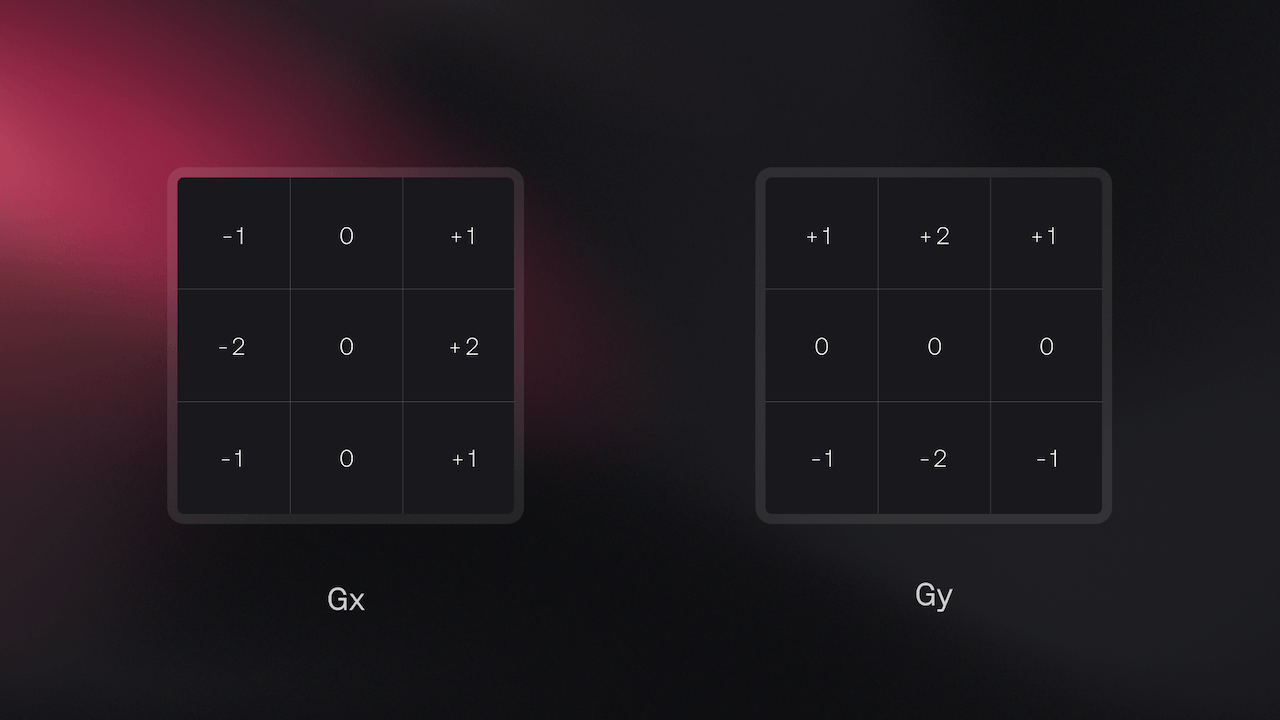
Next, let's introduce the concept of a “kernel”, these can also be referred to as “filters”; these are small grids (that can be a square or a rectangle) with numbers in it. These numbers are not random but are instead specifically picked to detect a certain feature. For example, a filter we could use to detect edges is the sobel edge detector.

Now you have both the image as luminance values and this kernel perform the following steps:

You will overlay the kernel over start of the image Next you will times each luminance pixel with the part of the grid it corresponds to in the kernel and then add up the sum of all these numbers Next you will slide this kernel one pixel to the side performing the same operation as the previous step. Each time you perform this operation you are creating a new pixel to create a new image Once you've slid the kernel across the entire image and you have all these new values, you can create a new image from these values. This new image is called the “feature map” and if you use this edge kernel it will highlight all the edges in the image.

There are different kernels to compute loads of different features and they aren't always a square, sometimes they are rectangular and they can be as big or small as you want, but keep in mind that bigger kernels result in more computation.

Convolutions aren't only used for things like edge detection but are extremely common in the image processing world, for tools you've probably used loads without even thinking about it, such as blurring images, sharpening and embossing.

Applications of Computer Vision

Now you have a good understanding of both the history and fundamentals of computer vision, you can dive into our other guides where we provide an even deeper dive into the different types of computer vision and how to implement them in your Appwrite application.